Google Sheets has evolved far beyond a simple spreadsheet tool. Today, it powers business reporting, marketing dashboards, financial planning, HR tracking, project management, automation workflows, and even lightweight data analysis.
At the heart of Google Sheets lies one powerful feature: formulas.
Whether you're calculating monthly expenses, analyzing campaign performance, tracking employee attendance, or building automated dashboards, Google Sheets formulas help you work faster, smarter, and more accurately.
The best part? You don’t need to be a spreadsheet expert to start.
This beginner-to-advanced Google Sheets formulas guide will teach you everything from basic spreadsheet formulas to advanced automation functions used by professionals and data analysts.
By the end of this guide, you’ll understand:
- What Google Sheets formulas are
- How formulas and functions work
- Essential beginner formulas
- Intermediate lookup and filtering functions
- Advanced automation formulas
- Common errors and troubleshooting
- Real-world use cases for businesses and professionals
- Best practices for building scalable spreadsheets
What Are Google Sheets Formulas?
Google Sheets formulas are built-in commands that help you perform calculations, automate tasks, analyze data, and manage information efficiently inside spreadsheets.
Instead of calculating values manually, formulas allow Google Sheets to do the work automatically using mathematical operators, functions, and cell references.
Formulas vs. Functions: What's the Difference?
These two terms get mixed up constantly, so let's clear it up.
A formula is the full expression you type into a cell, everything from the “=” sign to the closing “)”. A function is the pre-built operation within that formula, like SUM, AVERAGE, or IF. Think of a function as the tool, and the formula as the complete instruction using that tool.
So =SUM(B2:B20) is a formula. SUM is the function inside it.
The Anatomy of a Formula
Every Google Sheets formula has the same three-part structure:
- The equals sign (=): Always comes first. Without it, Google Sheets treats your input as plain text.
- The function name: Tells Sheets what operation to perform (e.g., SUM, IF, VLOOKUP).
- The arguments: The inputs inside the parentheses — usually cell references, ranges, or values that the function needs to do its job.
For example, in =AVERAGE(C2:C50), the function is AVERAGE and the argument is the range C2:C50.
Why Google Sheets Formulas Are Used
Google Sheets formulas are essential because they help users work more efficiently by automating calculations, reducing manual effort, and improving accuracy. Instead of calculating data manually every time information changes, formulas instantly update results automatically, saving time and minimizing human errors.
Benefits of Using Google Sheets Formulas
Automation
Formulas automatically update results whenever data changes, helping users save time and maintain accurate calculations without manual updates.
Productivity
Instead of spending hours performing manual calculations, Google Sheets formulas automate tasks and generate results within seconds.
Accuracy
Automated calculations reduce human errors and improve the accuracy and reliability of spreadsheet data.
Data Analysis
Formulas help users identify trends, analyze data, calculate averages, track growth rates, and uncover meaningful patterns more efficiently.
Reporting
Businesses use formulas to generate dynamic reports that automatically update whenever new data is added or modified.
Dashboard Creation
Advanced formulas help create interactive dashboards and KPI tracking systems that provide real-time business insights and performance monitoring.
How to Implement Formulas in Google Sheets
Knowing what formulas are is one thing. Putting them to work is another. Here's exactly how to do it.
Step-by-Step: Entering Your First Formula
- Click on the cell where you want the result to appear.
- Type = to start the formula.
- Type the function name (e.g., SUM). Google Sheets will show a dropdown of matching functions as you type, you can select one with the arrow keys and press Tab.
- Open a parenthesis “(“ and specify your range or values.
- Close the parenthesis “)” and press Enter.
Your result appears in the cell. That's your first formula.
Using Cell References vs. Hardcoded Values
You can write =SUM(100, 200) and it'll return 300. But that's rarely useful. The real power comes from referencing cells: =SUM(A1:A10). This way, if any value in A1 to A10 changes, your formula updates automatically.
Always use cell references instead of typing raw numbers into formulas. It keeps your spreadsheet dynamic and easy to maintain.
Understanding Cell References
A cell reference is the address of a cell in a spreadsheet. It tells Google Sheets where to find the data you want to use in a formula.
For example:
| Cell Reference | Meaning |
| A1 | Column A, Row 1 |
| B5 | Column B, Row 5 |
| C10 | Column C, Row 10 |
So when you write:
=A1+B1
Google Sheets looks at the values inside cells A1 and B1, then adds them together.
Types of Cell References
| Reference Type | Example | What It Does |
| Relative | A1 | Changes when you copy the formula to another cell |
| Absolute | $A$1 | Always refers to cell A1, no matter where you copy it |
| Mixed | $A1 or A$1 | Locks either the column or the row |
Copying and Dragging Formulas Down a Column
Once you write a formula in one cell, you don't have to retype it for every row. Click the cell with your formula, hover over the small blue square in the bottom-right corner, and drag it down. Google Sheets automatically adjusts the cell references for each row.
Using the Formula Bar
The formula bar appears above the spreadsheet.
You can:
- Edit formulas
- View long formulas
- Debug errors
- Understand calculations
Formatting Tips
Good formatting improves readability.
Use:
- Bold headers
- Borders
- Color coding
- Currency formatting
- Date formatting
- Conditional formatting
Google Sheets Formula Categories
Google Sheets organises its 500+ functions into 12 official categories. You don't need to learn all of them, but knowing what each category does helps you find the right tool faster when you need it.
Math & Arithmetic Formulas
These are the workhorses of any spreadsheet. Math and arithmetic functions handle all numerical calculations, from basic addition to rounding, absolute values, and square roots.
Key functions: SUM, PRODUCT, ROUND, MOD, ABS, SQRT, POWER
Example: =ROUND(A2*1.18, 2) multiplies a value by 1.18 (adding 18% tax) and rounds the result to 2 decimal places.
Text & String Formulas
Text functions let you manipulate, clean, and extract text from cells. They're essential when you're working with imported data, building URLs, formatting names, or combining values into readable strings.
Key functions: TRIM, CONCATENATE, LEFT, RIGHT, MID, UPPER, LOWER, LEN, SUBSTITUTE
Example: =PROPER(A2) converts "john smith" into "John Smith" — useful for cleaning up messy name data.
Logical Formulas
Text functions let you manipulate, clean, and extract text from cells. They're essential when you're working with imported data, building URLs, formatting names, or combining values into readable strings.
Key functions: TRIM, CONCATENATE, LEFT, RIGHT, MID, UPPER, LOWER, LEN, SUBSTITUTE
Example: =PROPER(A2) converts "john smith" into "John Smith", which is useful for cleaning up messy name data.
Lookup & Reference Formulas
Logical functions let you build conditions into your spreadsheet. They test whether something is true or false and return different results based on the outcome. This is where your spreadsheet starts making decisions for you.
Key functions: IF, IFS, AND, OR, NOT, IFERROR, IFNA
Example: =IF(AND(B2>50, C2="Active"), "Eligible", "Not Eligible") checks two conditions at once and returns the appropriate label.
Date & Time Formulas
These functions search your data and pull values from elsewhere in the spreadsheet. They're the backbone of any sheet that connects multiple data sources or tables.
Key functions: VLOOKUP, HLOOKUP, INDEX, MATCH, XLOOKUP, OFFSET, INDIRECT
Example: =INDEX(B2:B100, MATCH(E2, A2:A100, 0)) finds a value more flexibly than VLOOKUP. It searches in any direction and doesn't break when you insert columns.
Statistical Formulas
Statistical functions go beyond simple averages. They help you analyse distributions, find outliers, measure variance, and understand the shape of your data. They're useful for anyone working with survey results, test scores, or performance data.
Key functions: AVERAGE, MEDIAN, MODE, STDEV, VAR, COUNT, COUNTA, COUNTBLANK, PERCENTILE
Example: =MEDIAN(B2:B100) returns the middle value in a dataset. It's often more useful than AVERAGE when your data has extreme outliers.
Array Formulas
Array formulas apply a calculation across an entire range of cells at once, without needing to copy the formula into every row. They're powerful for automation and reducing repetitive work.
Key functions: ARRAYFORMULA, FILTER, UNIQUE, SORT, TRANSPOSE
Example: =ARRAYFORMULA(A2:A100 * B2:B100) multiplies every value in column A by the corresponding value in column B across 99 rows with a single formula.
Google-Specific Formulas
These are functions you won't find in Excel. They're built exclusively for Google Sheets and tap into Google's ecosystem by pulling live data from the web, translating text, or importing data from other spreadsheets.
Key functions: IMPORTRANGE, GOOGLEFINANCE, GOOGLETRANSLATE, IMAGE, SPARKLINE, QUERY
Example: =GOOGLEFINANCE("AAPL", "price") pulls Apple's live stock price directly into your sheet without manual updates.
Financial Formulas
Financial functions are designed for money-related calculations, including loan repayments, investment returns, depreciation, and cash flow analysis. They're built for accountants, analysts, and anyone managing budgets or forecasting.
Key functions: PMT, NPV, IRR, FV, PV, RATE, SLN, DB
Example: =PMT(0.05/12, 60, -10000) calculates the monthly payment on a $10,000 loan at 5% annual interest over 5 years.
Database Formulas
Database functions work like mini SQL queries on a structured table. They let you sum, count, or average values based on complex multi-condition criteria, much like a pivot table but inside a formula.
Key functions: DSUM, DCOUNT, DAVERAGE, DMAX, DMIN, DGET
Example: =DSUM(A1:D100, "Revenue", F1:G2) adds up revenue from a table based on criteria you define in a separate range. This is useful for advanced conditional aggregations.
Information Formulas
Information functions check what type of data is inside a cell and return TRUE or FALSE. They're especially useful for data validation, error-proofing your formulas, and building logic around incomplete datasets.
Key functions: ISNUMBER, ISTEXT, ISBLANK, ISERROR, ISNA, ISODD, ISEVEN, TYPE
Example: =ISBLANK(A2) returns TRUE if cell A2 is empty. You can use this inside an IF formula to handle missing data without breaking your sheet.
Engineering Formulas
Engineering functions handle number base conversions and bitwise operations. They're niche and primarily used by developers, engineers, and data professionals working with binary, hexadecimal, or octal number systems.
Key functions: BIN2DEC, DEC2BIN, HEX2DEC, DEC2HEX, OCT2DEC, BITAND, BITOR, BITXOR
Example: =HEX2DEC("FF") converts the hexadecimal value FF into the decimal number 255. This is useful when working with colour codes or low-level data formats.
Where to start:
If you're a beginner, focus on Math, Text, Logical, and Lookup categories first. Those four will cover 80% of what most people need from Google Sheets. The rest you can explore as your work demands it.
Top 10 Most Useful Google Sheets Formulas
These aren't just the most popular formulas. Each one covers a completely different use case. Together, they can handle the majority of what you'll ever need from Google Sheets.
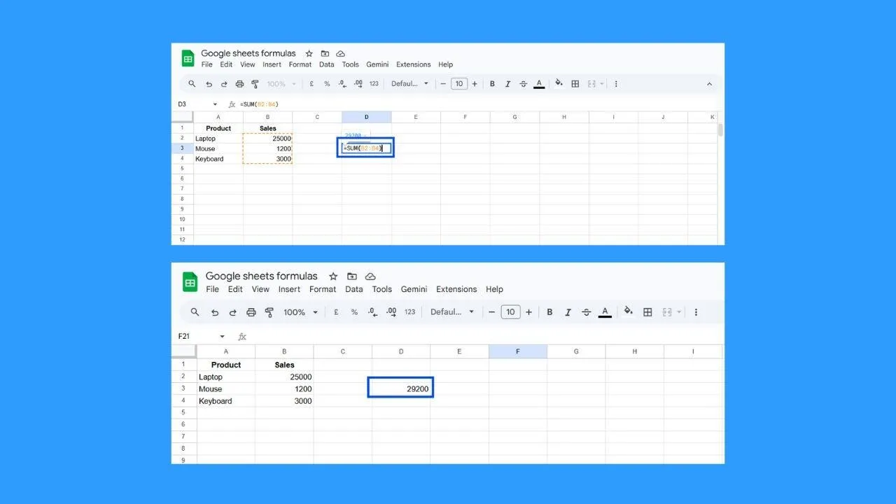
SUM: Basic Calculation Foundation
What it does: Adds up all values in a range. It's the most used formula in any spreadsheet, period.
Syntax: =SUM(range)
Example: =SUM(B2:B100) instantly totals every sales figure in column B without you touching a calculator. Change any value in that range and the total updates automatically.
IF: Logical Decision-Making
What it does: Tests a condition and returns one value if it's true and another if it's false. This is the formula that makes your spreadsheet think.
Syntax: =IF(condition, value_if_true, value_if_false)
Example: =IF(D2>=50, "Pass", "Fail") evaluates a student's score and labels it automatically. You can also nest IF inside IF to handle multiple conditions, though for complex logic, IFS is cleaner.

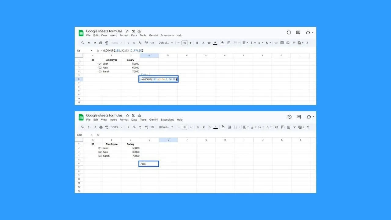
VLOOKUP: Data Retrieval
What it does: Searches for a value in the first column of a table and returns a related value from another column in the same row. Think of it as a search engine for your data.
Syntax: =VLOOKUP(search_key, range, index, is_sorted)
Example: =VLOOKUP(A2, Products!A:C, 2, FALSE) looks up a product ID in A2 and pulls the matching product name from your Products sheet. Always use FALSE as the last argument to get an exact match.
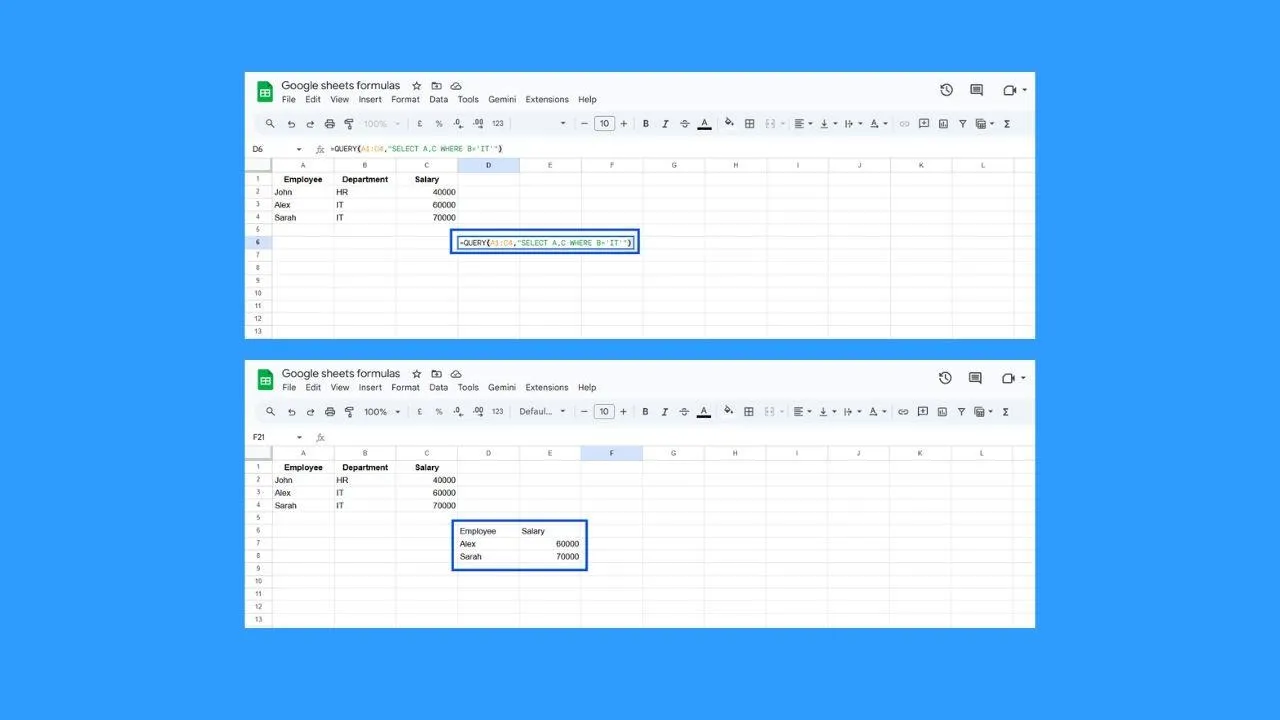
QUERY: Advanced Analysis
What it does: Lets you run SQL-style queries on your data by filtering, sorting, grouping, and summarising all in one formula. It's the most powerful Google-specific formula most beginners don't discover until much later.
Syntax: =QUERY(data, query, headers)
Example: =QUERY(A1:D100, "SELECT A, B, D WHERE C = 'North' ORDER BY D DESC", 1) pulls only the rows where the region is North, returns three specific columns, and sorts by the last column, all without touching filters or pivot tables.
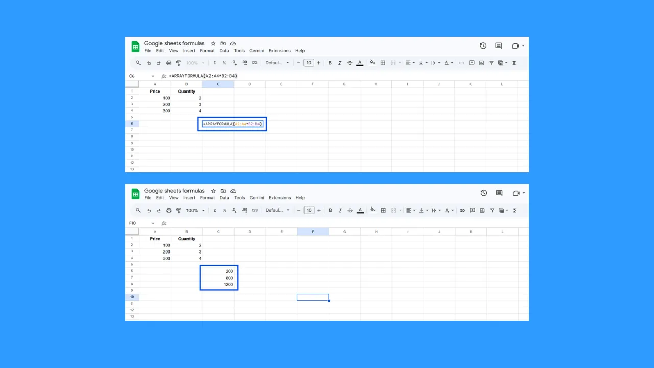
ARRAYFORMULA: Automation
What it does: Applies a formula to an entire column or range at once instead of copying it row by row. One formula does the work of hundreds.
Syntax: =ARRAYFORMULA(formula)
Example: =ARRAYFORMULA(A2:A100 * B2:B100) multiplies every value in column A by the corresponding value in column B across all 99 rows simultaneously. If you add new data, it calculates automatically without dragging formulas down.
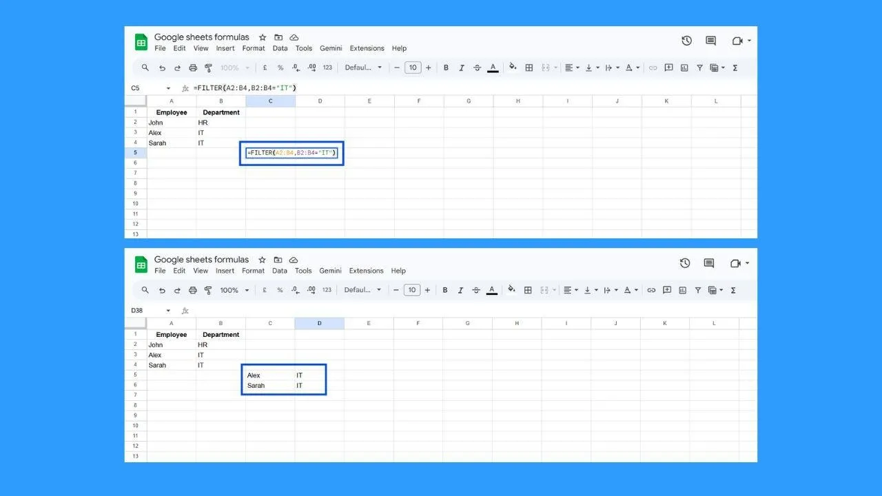
FILTER: Dynamic Reporting
What it does: Returns only the rows that meet one or more conditions, creating a live filtered view of your data. Unlike manual filters, FILTER outputs results into a new range and updates dynamically as your data changes.
Syntax: =FILTER(range, condition1, condition2, ...)
Example: =FILTER(A2:D100, C2:C100="Completed") pulls all rows where the status column says "Completed". It's perfect for building dynamic dashboards or live task trackers.
UNIQUE: Duplicate Removal
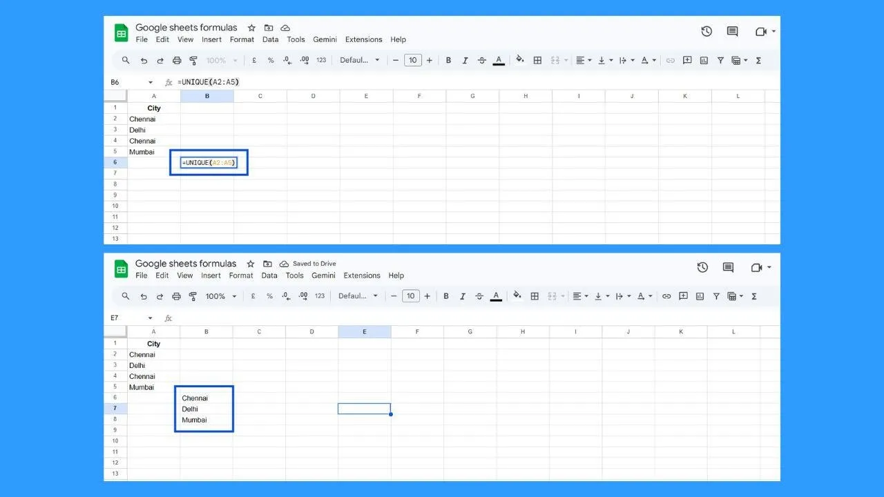
What it does: Returns a list with all duplicate values removed, keeping only distinct entries. Simple, but incredibly useful when cleaning data or building dropdown lists.
Syntax: =UNIQUE(range)
Example: =UNIQUE(A2:A200) takes a column of 200 customer names, many repeated, and outputs a clean list of unique names only. Combine it with SORT for an alphabetically ordered unique list: =SORT(UNIQUE(A2:A200)).
COUNTIF: Conditional Analysis
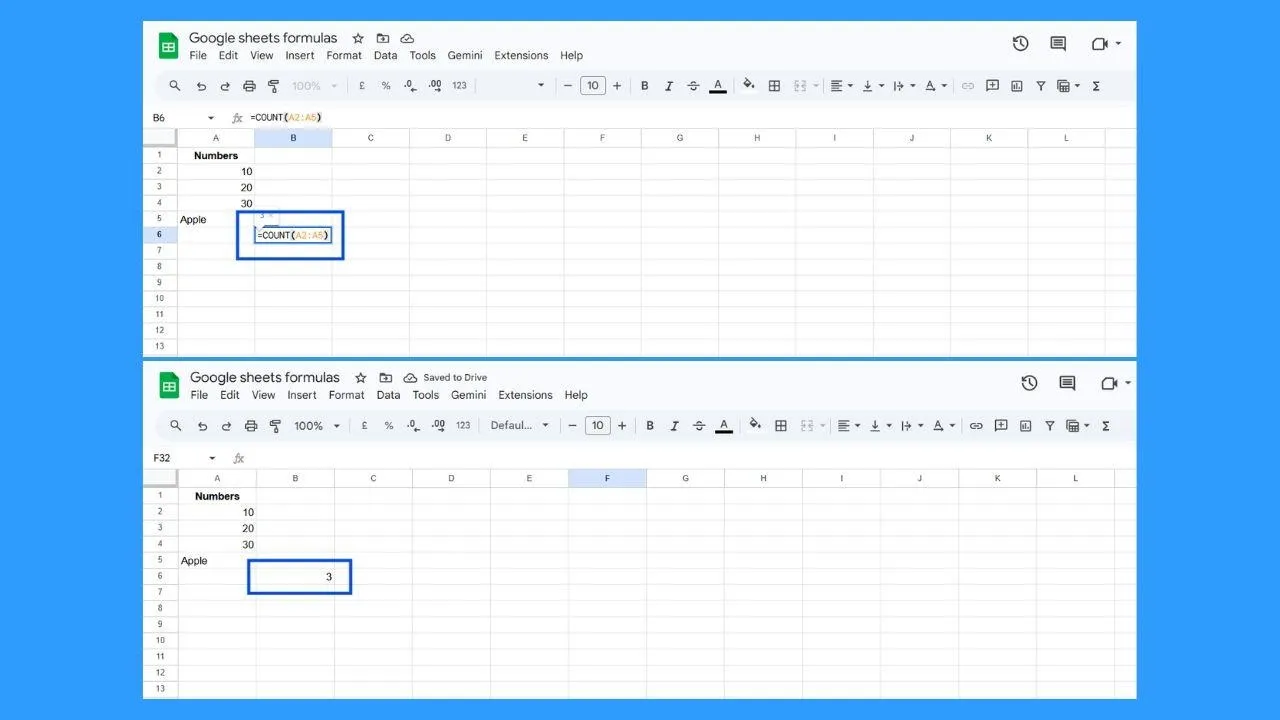
What it does: Counts the number of cells in a range that meet a specific condition. It's the quickest way to answer the question, “How many of these exist in my data?”
Syntax: =COUNTIF(range, criteria)
Example: =COUNTIF(E2:E200, "Pending") counts exactly how many tasks are still pending in your tracker. You can use wildcards too. =COUNTIF(A2:A100, "John*") counts every name that starts with John.
IFERROR: Error Handling
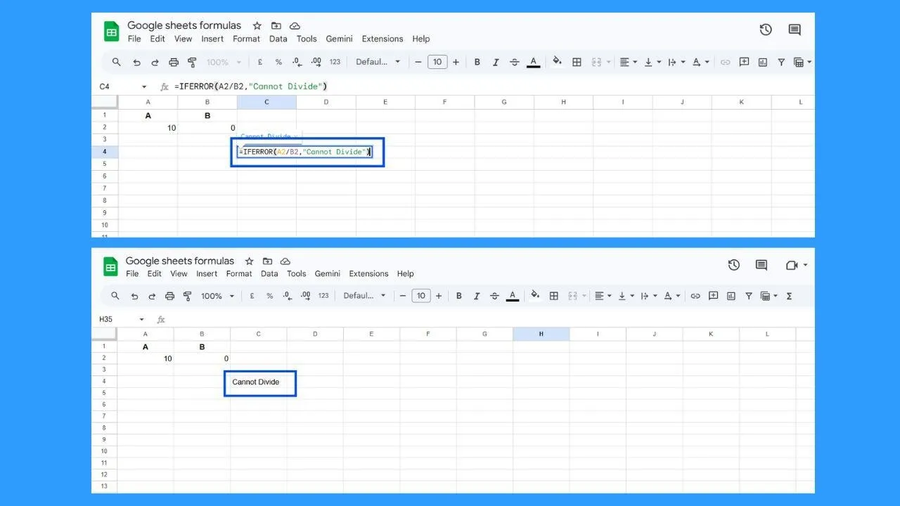
What it does: Wraps around any formula and catches errors before they show up as ugly codes like #N/A or #REF!. Instead, it displays a value you choose, making your sheet look clean and professional.
Syntax: =IFERROR(formula, value_if_error)
Example: =IFERROR(VLOOKUP(A2, B:C, 2, FALSE), "Not Found") shows "Not Found" instead of #N/A when a lookup fails. Wrap any formula that could potentially error, especially VLOOKUPs, divisions, and IMPORTRANGEs.
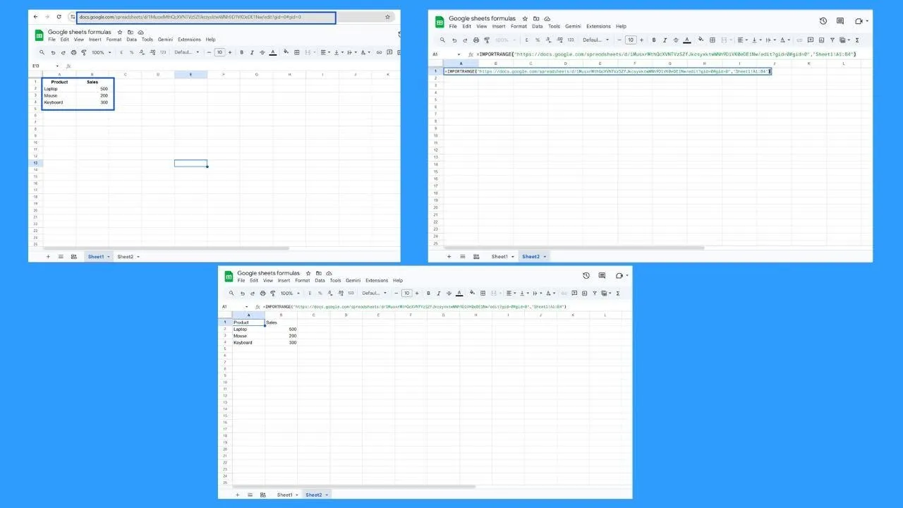
IMPORTRANGE: Cross-Sheet Workflows
What it does: Pulls data from a completely separate Google Sheets file into your current sheet live. This is a Google Sheets-exclusive formula with no real Excel equivalent, and it's what makes multi-sheet workflows possible.
Syntax: =IMPORTRANGE("spreadsheet_url", "sheet!range")
Example: =IMPORTRANGE("https://docs.google.com/spreadsheets/d/YOUR_ID", "Sheet1!A1:D100") imports a live data range from another file. Any updates made in the source file appear automatically in your sheet without copy-pasting between files.
Common Formula Errors and How to Fix Them
Every Google Sheets user hits errors. They're not a sign something's broken beyond repair. They're simply feedback. Here's what the most common formula errors in Google Sheets mean and how to fix them fast.
#DIV/0!
What it means: You're dividing by zero or by an empty cell.
Fix: Wrap your formula in IFERROR, or use an IF statement to check that the denominator isn't zero before dividing.
Example
=IF(B2=0, 0, A2/B2)
#N/A
What it means: The value you're looking for doesn't exist in the specified range. This is most common with VLOOKUP and MATCH.
Fix: Double-check your search value for typos or extra spaces. Use TRIM to clean the data, then wrap the formula in IFERROR to handle cases where no match exists.
#REF!
What it means: A cell reference in your formula is no longer valid. This usually happens because you deleted a row or column that the formula was pointing to.
Fix: Press Ctrl+Z immediately to undo the deletion if possible. Otherwise, re-enter the correct cell range manually.
#NAME?
What it means: Google Sheets doesn't recognise something in your formula. This is usually caused by a misspelled function name, a missing quotation mark around text, or a named range that doesn't exist.
Fix: Check your function name for typos. Make sure text values are wrapped in quotation marks. Use the formula suggestions dropdown to select the correct function while typing.
#VALUE!
What it means: You're trying to perform a mathematical operation on a cell that contains text instead of a number.
Fix: Make sure all cells in your formula range contain the correct data type. Use IFERROR or IFNA to handle unexpected value types gracefully without breaking your sheet.
Understanding what formula parse errors mean goes a long way. Once you know what each error is telling you, fixing it becomes straightforward instead of a guessing game.
Best Practices for Writing Google Sheets Formulas
Knowing formulas is one skill. Writing them well is another. These habits will save you from headaches later.
Use Named Ranges for Clarity
Instead of referencing B2:B100 everywhere, name that range "MonthlySales" under Data > Named Ranges. Your formulas become much easier to read and understand briefly.
Lock References with $ When Copying Formulas
If part of your formula should never change, such as a reference to a fixed tax rate or a lookup table, use the dollar sign to anchor it.
Example
=$A$1
This prevents the reference from shifting when you drag the formula to other cells.
Always Wrap Risky Formulas in IFERROR
Any formula that could fail, especially LOOKUPs and division-based formulas, should have an IFERROR wrapper. It keeps your sheet clean and prevents one bad row from breaking the entire column.
Keep Formulas Short and Readable
If a formula becomes so long that you can't understand it quickly, break it into helper columns. Calculate intermediate steps separately, then reference those cells in your final formula. This makes debugging much easier later.
Use Consistent Data Formatting
Formulas break when data types are inconsistent. Make sure:
- Number columns contain only numbers
- Date columns are formatted as actual dates
- Text columns don't contain unnecessary spaces
The TRIM and TEXT functions are especially useful for cleaning messy data.
Conclusion
Google Sheets formulas aren't something you master overnight, but they're not nearly as intimidating as they first appear.
Here's what to take away from this guide: start with the fundamentals like SUM, AVERAGE, and IF. Once those feel natural, move on to VLOOKUP and COUNTIF. Then tackle IFERROR and ARRAYFORMULA to make your sheets more robust and automated.
Errors will happen. Now you know what they mean and how to fix them. Best practices will keep your formulas clean, readable, and reliable as your sheets grow.
The more you use formulas, the more second-nature they become. Open a sheet today, pick one formula from this guide, and try it on real data. That's the fastest way to go from staring at a blank cell to making Google Sheets work for you.
As your Google Sheets formulas start uncovering valuable insights, the next step is making that data easier to interpret and share. That’s where ChartApps can help. By connecting Google Sheets data with interactive charts, dashboards, and reporting workflows, ChartApps enables teams to present spreadsheet data in a more visual and organized way without a complicated setup.
Frequently Asked Questions
What are the most useful Google Sheets formulas?
SUM, IF, VLOOKUP, QUERY, FILTER, and ARRAYFORMULA are among the most useful formulas.
Which formulas should beginners learn first?
Beginners should focus on learning the most commonly used and practical formulas first. These formulas build the foundation for working efficiently in spreadsheets.
Some essential beginner formulas include:
- SUM – Adds numbers
- AVERAGE – Calculates averages
- COUNT – Counts numeric values
- IF – Creates logical conditions
- COUNTIF – Counts cells matching criteria
- VLOOKUP – Finds data from tables
- CONCATENATE or TEXTJOIN – Combines text
What is ARRAYFORMULA?
ARRAYFORMULA is an advanced Google Sheets function that applies a formula to an entire range of cells automatically instead of copying the formula row by row. It helps automate repetitive spreadsheet tasks and keeps formulas cleaner.
How do I automate tasks in Google Sheets?
You can automate spreadsheets in Google Sheets using formulas, functions, conditional formatting, pivot tables, and Google Apps Script. Automation reduces manual work, improves accuracy, and updates calculations instantly when data changes.
What are the best formulas for data analysis?
QUERY, FILTER, UNIQUE, INDEX MATCH, and ARRAYFORMULA are excellent for data analysis.