If you have ever copied the same formula down hundreds of rows in Google Sheets, you have probably wondered if there is a faster way to do it.
Maybe you created a sales sheet, entered one formula in row 2, then dragged it all the way to row 500. It works, but it also feels repetitive, fragile, and easy to break. One accidental deletion and the whole column become inconsistent. That is where array formulas come in.
Array formulas are one of the most powerful features in Google Sheets. They let you apply a single formula to an entire range of cells automatically. Once you understand how they work, you can build cleaner spreadsheets, automate repetitive calculations, and create dynamic reports that update themselves.
In this guide, you will learn array formulas from the ground up. We will start with the basics of what arrays are, then move into practical ARRAYFORMULA examples, conditional logic, advanced array functions, and real-world spreadsheet techniques used by power users.
What Is an Array Formula?
An array is simply a collection of values. Instead of working with one cell at a time, array formulas work with many cells at once.
For example:
- A regular formula might calculate A2 * B2
- An array formula can calculate A2:A100 * B2:B100 all in one step
Think of it like switching from handling one item manually to processing an entire batch automatically.
Google Sheets is especially good at handling arrays because many functions are built to support ranges natively.
List of Array Formulas in Google Sheets
| Type | Name | Syntax | Description |
| Array | ARRAY_CONSTRAIN | ARRAYCONSTRAIN(inputrange, numrows, numcols) | Trims an array output down to a specific number of rows and columns. Useful when a formula returns more results than you need to display. |
| Array | BYCOL | BYCOL(arrayorrange, LAMBDA) | Runs a custom LAMBDA function on each column of a range individually and returns one result per column. Great for getting column-level stats like sum or average without a helper row. |
| Array | BYROW | BYROW(arrayorrange, LAMBDA) | Runs a custom LAMBDA function on each row of a range individually and returns one result per row. Perfect for row-wise totals or custom calculations without helper columns. |
| Array | CHOOSECOLS | CHOOSECOLS(array, colnum1, [colnum2]) | Picks specific columns from a range and returns them as a new array. Lets you reorder or extract only the columns you need without rearranging your source data. |
| Array | CHOOSEROWS | CHOOSEROWS(array, rownum1, [rownum2]) | Picks specific rows from a range and returns them as a new array. Useful for pulling out selected records by position. |
| Array | FLATTEN | FLATTEN(range1,[range2,...]) | Collapses multiple ranges or a multi-dimensional array into a single flat column of values. Handy when combining data from different ranges into one list. |
| Array | FREQUENCY | FREQUENCY(data, classes) | Counts how many values fall within each defined range or "bin." Commonly used to build histograms or score distribution tables. |
| Array | GROWTH | GROWTH(knowndatay, [knowndatax], [newdatax], [b]) | Fits an exponential growth curve to your existing data and uses it to predict future values. Useful for forecasting revenue, user growth, or any metric that compounds over time. |
| Array | HSTACK | HSTACK(range1; [range2, …]) | Joins multiple ranges side by side horizontally into one wider array. Ideal for combining columns from different parts of a sheet into a single table. |
| Array | LINEST | LINEST(knowndatay, [knowndatax], [calculate_b], [verbose]) | Calculates the parameters of the best-fit straight line through your data using the least-squares method. Used in regression analysis and trend modeling. |
| Array | LOGEST | LOGEST(knowndatay, [knowndatax], [b], [verbose]) | Similar to LINEST but fits an exponential curve instead of a straight line. Used when your data grows or declines at a percentage rate rather than a fixed amount. |
| Array | MAKEARRAY | MAKEARRAY(rows, columns, LAMBDA) | Generates a new array of a specified size where each cell value is calculated by a LAMBDA function. Useful for building dynamic tables or grids from scratch without source data. |
| Array | MAP | MAP(array1, [array2, ...], LAMBDA) | Applies a LAMBDA function to every individual value in an array and returns a transformed array of the same size. Perfect for custom calculations like applying tax rates, markups, or formatting rules across a range. |
| Array | MDETERM | MDETERM(square_matrix) | Returns the mathematical determinant of a square matrix. Primarily used in advanced linear algebra and engineering calculations. |
| Array | MINVERSE | MINVERSE(square_matrix) | Returns the inverse of a square matrix. Used in solving systems of linear equations and advanced mathematical modeling. |
| Array | MMULT | MMULT(matrix1, matrix2) | Multiplies two matrices together and returns the resulting matrix. Useful for weighted scoring, financial modeling, and any multi-variable calculation that involves matrix math. |
| Array | REDUCE | REDUCE(initialvalue, arrayor_range, LAMBDA) | Processes every value in an array one by one, accumulating a running result using a LAMBDA function, and returns a single final value. Think of it as a custom version of SUM or PRODUCT with your own logic. |
| Array | SCAN | SCAN(initialvalue, arrayor_range, LAMBDA) | Similar to REDUCE but returns all the intermediate accumulated values instead of just the final result. Useful for building running totals, cumulative counts, or step-by-step progressions. |
| Array | SUMPRODUCT | SUMPRODUCT(array1, [array2, ...]) | Multiplies corresponding values across two or more arrays and returns the sum of all those products. One of the most versatile functions in Sheets, commonly used for weighted averages, revenue calculations, and conditional summing. |
| Array | SUMX2MY2 | SUMX2MY2(arrayx, arrayy) | Calculates the sum of the differences between the squares of two arrays (x² - y²). Used in statistical and engineering calculations. |
| Array | SUMX2PY2 | SUMX2PY2(arrayx, arrayy) | Calculates the sum of the sums of the squares of two arrays (x² + y²). Used in statistical distance and error calculations. |
| Array | SUMXMY2 | SUMXMY2(arrayx, arrayy) | Calculates the sum of the squared differences between two arrays ((x - y)²). Commonly used in measuring variance or error between predicted and actual values. |
| Array | TOCOL | TOCOL(arrayorrange, [ignore], [scanbycolumn]) | Converts a multi-row, multi-column range into a single vertical column. Useful for flattening a table into a list for further processing. |
| Array | TOROW | TOROW(arrayorrange, [ignore], [scanbycolumn]) | Converts a multi-row, multi-column range into a single horizontal row. The counterpart to TOCOL when you need data laid out across columns instead. |
| Array | TRANSPOSE | TRANSPOSE(arrayorrange) | Flips a range so rows become columns and columns become rows. A quick way to reorient data without manually rearranging it. |
| Array | TREND | TREND(knowndatay, [knowndatax], [newdatax], [b]) | Fits a straight-line trend to your existing data and predicts future values along that line. Used for linear forecasting in sales, budgeting, and performance tracking. |
| Array | VSTACK | VSTACK(range1; [range2, …]) | Joins multiple ranges on top of each other vertically into one taller array. Ideal for combining data from multiple sheets or tables into a single consolidated list. |
| Array | WRAPCOLS | WRAPCOLS(range, wrapcount, [padwith]) | Takes a flat list and wraps it into multiple columns after a set number of values. Useful for reshaping a long list into a grid layout. |
| Array | WRAPROWS | WRAPROWS(range, wrapcount, [padwith]) | Takes a flat list and wraps it into multiple rows after a set number of values. The row-based counterpart to WRAPCOLS for building grid layouts from lists. |
Now, let's dive into a detailed look at ArrayFormula in Google Sheets. Before starting, Use this sample dataset below to practice the ArrayFormula feature in Google Sheets.
How Array Formulas Differ from Regular Formulas
A regular formula usually returns one result in one cell.
Example:
This only calculates a single row.
An array formula can return multiple results across many rows automatically.
Example:
=ARRAYFORMULA(A2:A10+B2:B10)
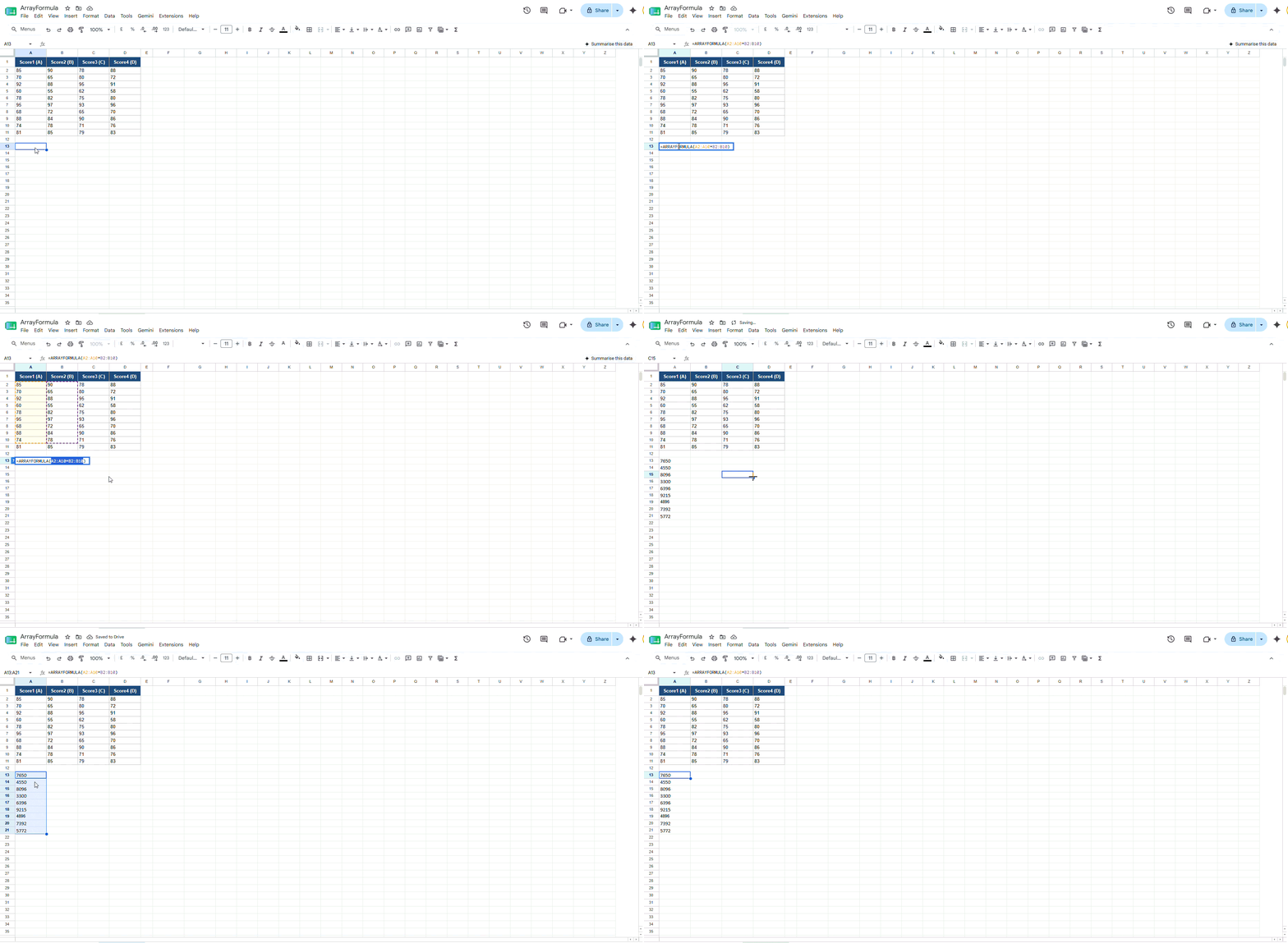
This formula calculates every matching row between columns A and B at once.
Instead of copying the formula down manually, one formula fills the entire result column.
Ctrl+Shift+Enter vs ARRAYFORMULA
In older spreadsheet programs like Microsoft Excel, array formulas were often entered using Ctrl+Shift+Enter.
Google Sheets supports this shortcut too, but most users today use the ARRAYFORMULA function directly because it is clearer and easier to manage.
Example:
=ARRAYFORMULA(A2:A10*B2:B10)
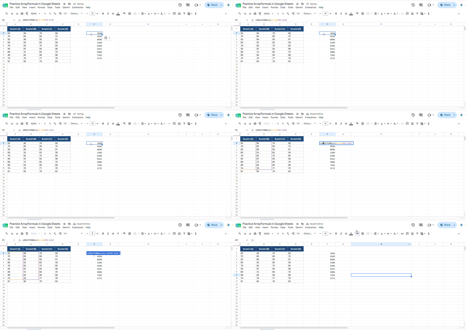
This is the modern and recommended approach in Google Sheets.
What Curly Braces {} Mean
Curly braces in Google Sheets are used to manually create literal arrays, making it easy to organize and combine data dynamically.
For example, using ={1,2,3} creates a horizontal array where the values appear across a single row, while ={1;2;3} creates a vertical array with the values stacked in a single column.
Curly braces can also be used to merge ranges together, such as ={A2:A10,B2:B10}, which combines two columns side by side into a new array. This feature is especially useful when building custom outputs, restructuring datasets, or combining information from multiple ranges into one unified result.
ARRAYFORMULA Basics
Replacing Repetitive Calculations
The biggest advantage of ARRAYFORMULA is automation.
Instead of filling formulas row by row, one formula handles the entire column.
Basic Arithmetic with ARRAYFORMULA
ARRAYFORMULA in Google Sheets makes it possible to apply arithmetic operations across an entire range without manually dragging formulas down row by row.
Normally, if you want to multiply two cells, you would use a formula like =A2*B2 and then copy it downward for the rest of the dataset.
With ARRAYFORMULA, you can handle the entire column at once using =ARRAYFORMULA(A2:A100*B2:B100). This formula automatically multiplies each value in column A with its corresponding value in column B and returns all the results in a single step.
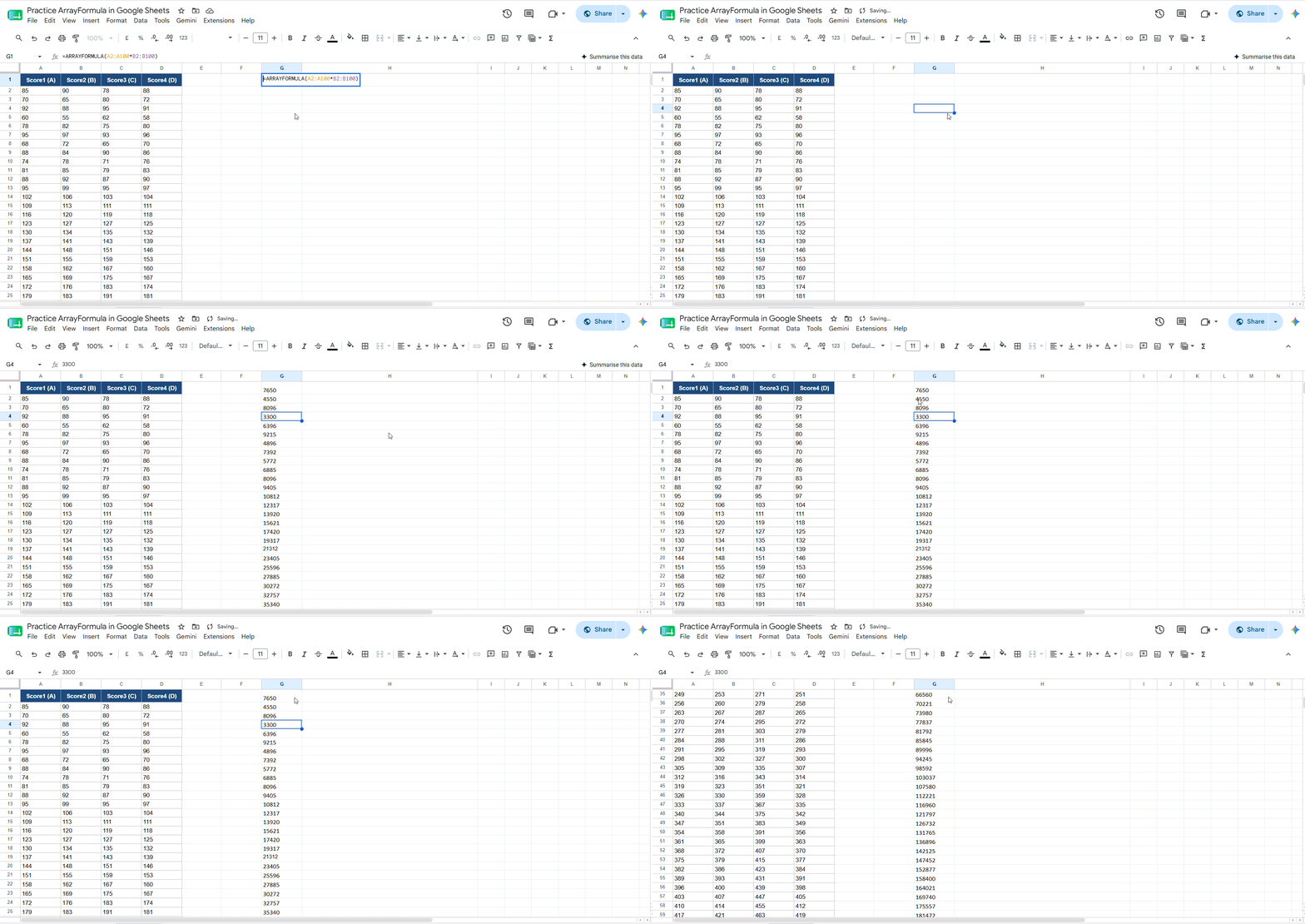
It is especially useful for tasks like calculating total sales, where one column contains quantities and another contains unit prices, allowing the formula to update dynamically as new rows are added.
Using IF Logic Across a Range
ARRAYFORMULA can also be combined with logical functions like IF to apply conditions across an entire dataset automatically. Normally, you would write a formula such as =IF(C2="Yes","Approved","Pending") and then drag it down through the column.
With an array formula, you can process all rows at once using =ARRAYFORMULA(IF(C2:C100="Yes","Approved","Pending")).
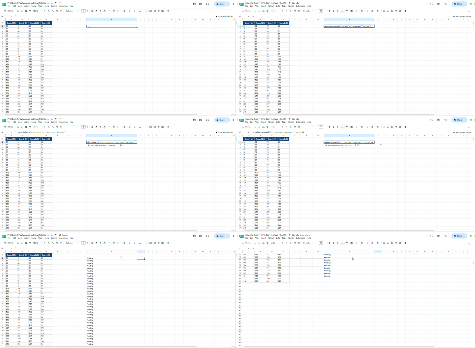
This formula checks every cell in column C and returns "Approved" whenever the value is "Yes"; otherwise, it returns "Pending". It is particularly useful in workflow or tracking sheets where statuses need to update automatically for large numbers of entries without requiring manual copying of formulas.
Applying Text Functions Across Multiple Rows
ARRAYFORMULA is also useful for applying text functions across multiple rows automatically. Normally, to convert text into uppercase, you would use a formula like =UPPER(A2) and then drag it down the column for every row.
With an array formula, you can process the entire range at once using =ARRAYFORMULA(UPPER(A2:A100)).
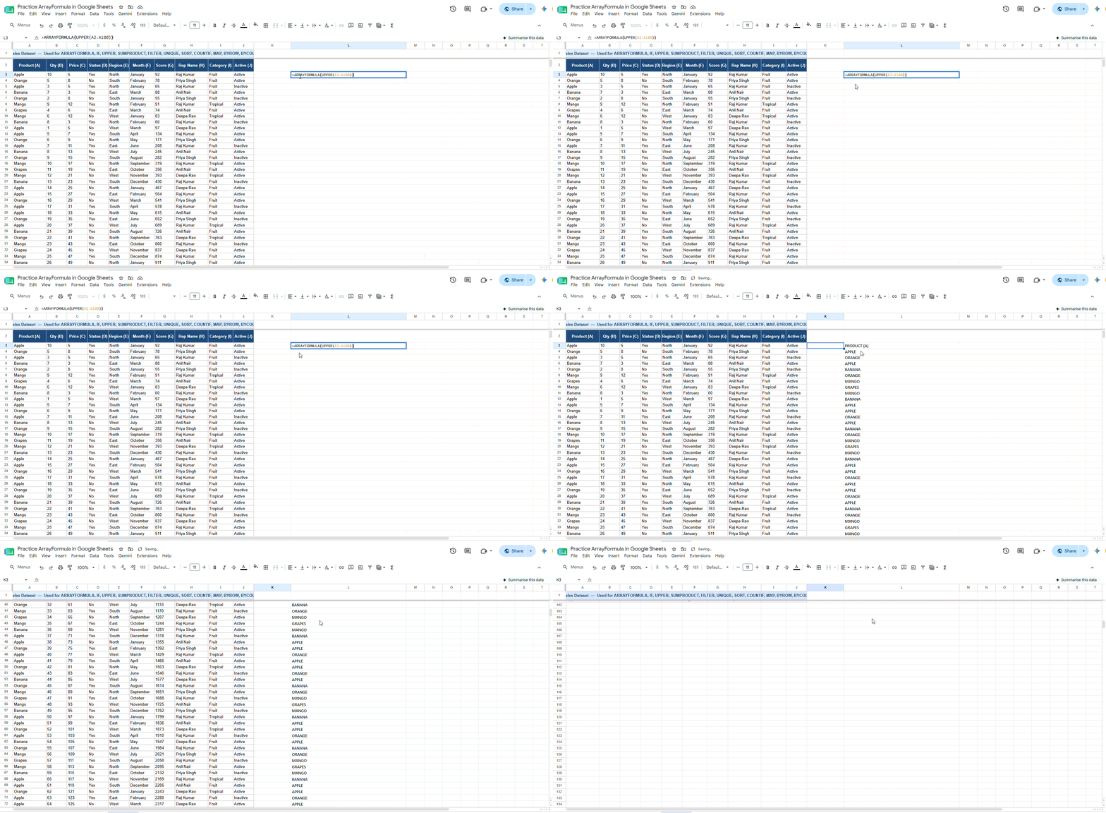
This formula converts every text value in the selected range into uppercase automatically, without needing to copy the formula manually. It is especially helpful when standardizing customer names, product codes, or any text-based data to maintain consistent formatting throughout a dataset.
Combining Columns Automatically
ARRAYFORMULA can also be used to combine data from multiple columns into a single formatted output automatically.
For example, the formula =ARRAYFORMULA(A2:A100&" - "&B2:B100) joins the values from column A and column B with a hyphen separator in between.
Instead of writing the formula row by row, the array formula processes the entire range at once and generates combined results for every matching row automatically.
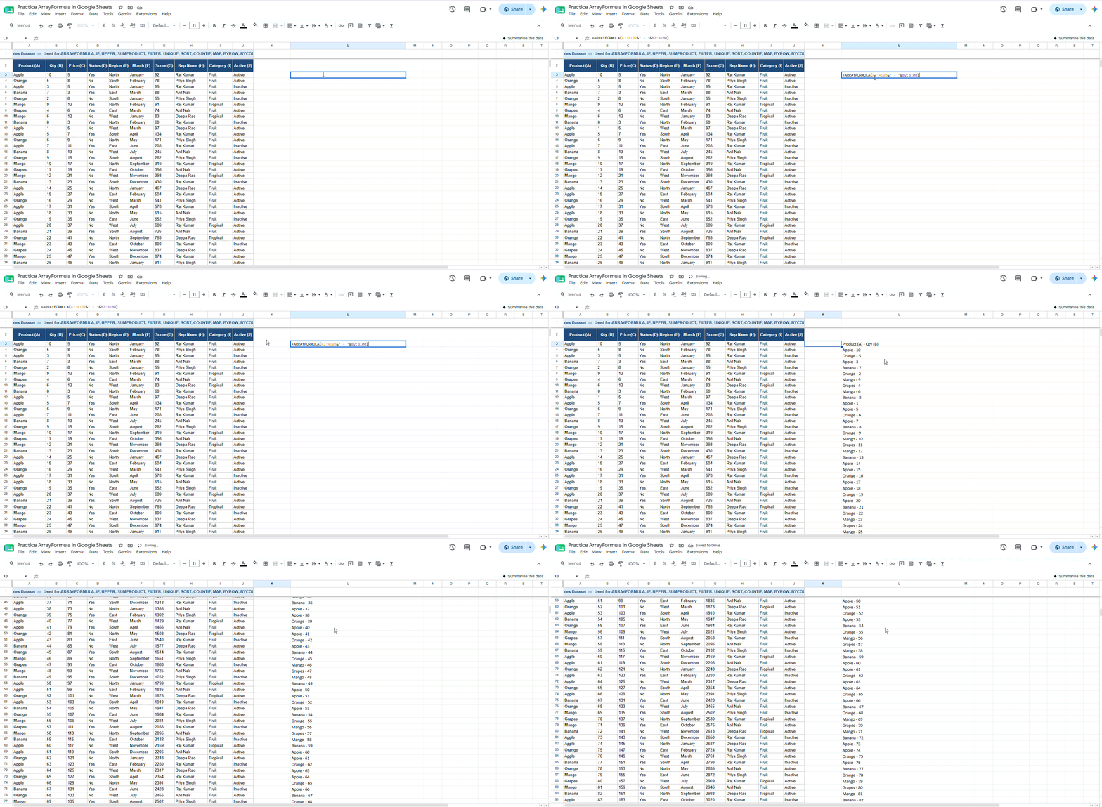
This is especially useful for creating structured labels such as "Product Name - Category", combining first and last names, or generating custom identifiers in large datasets.
Preventing Blank Row Errors
One common challenge with ARRAYFORMULA is that it may continue displaying results or errors even in empty rows. To avoid this, you can combine ARRAYFORMULA with an IF condition for cleaner outputs.
For example, the formula =ARRAYFORMULA(IF(A2:A100="","",A2:A100*B2:B100)) first checks whether the cells in column A are empty. If a row has no data, it returns a blank cell instead of performing the calculation.
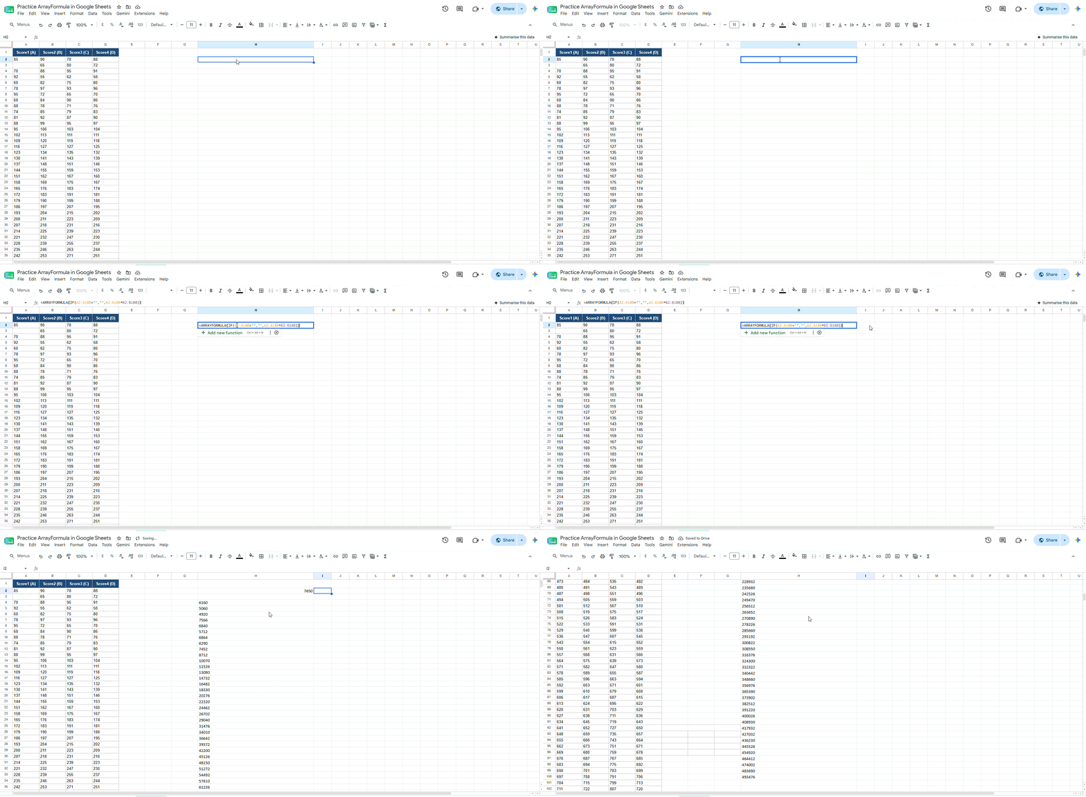
If data exists, it multiplies the corresponding values from columns A and B. This approach is especially useful in large spreadsheets because it keeps the sheet visually clean, prevents unnecessary errors, and ensures formulas only appear where actual data is present.
Arrays with Lookup and Aggregation Functions
SUMPRODUCT
SUMPRODUCT is a powerful Google Sheets function that multiplies corresponding values from multiple arrays and then adds all the results together into a single total.
For example, the formula =SUMPRODUCT(A2:A10,B2:B10) takes each value in column A, multiplies it by the matching value in column B, and then sums all the calculated products.
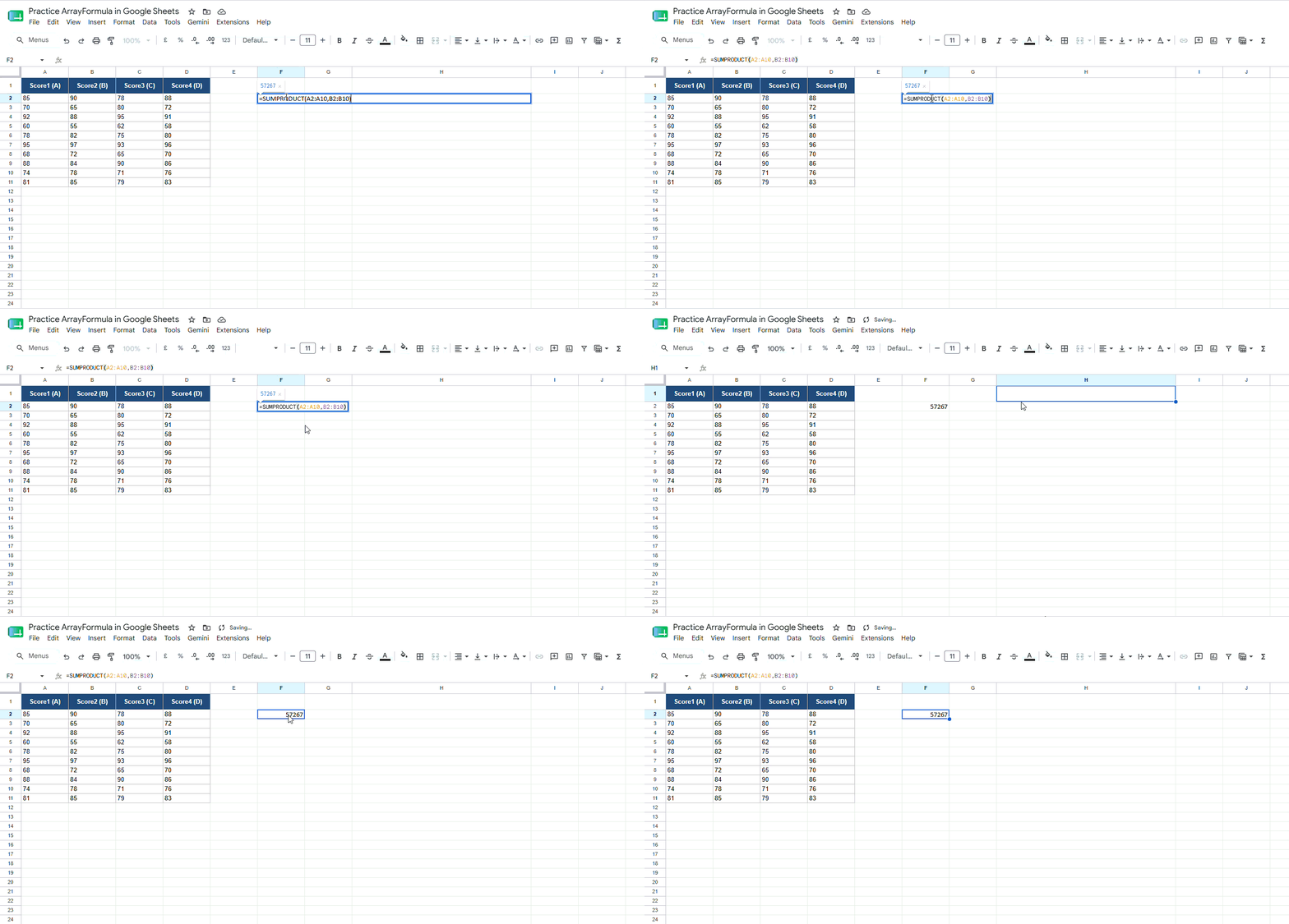
This makes it extremely useful for tasks like calculating total revenue, where one column contains quantities and another contains prices.
Instead of creating a separate column for individual calculations, SUMPRODUCT performs everything within a single formula.
The function becomes even more powerful when combined with conditions, allowing you to calculate totals based on specific criteria such as categories, dates, or statuses.
COUNTIF with Multiple Criteria
Google Sheets also supports using arrays inside counting functions, making it possible to evaluate multiple conditions within a single formula.
For example, the formula =SUM(COUNTIF(A2:A100,{"Apple","Orange"})) checks the range A2:A100 and counts how many times either "Apple" or "Orange" appears.
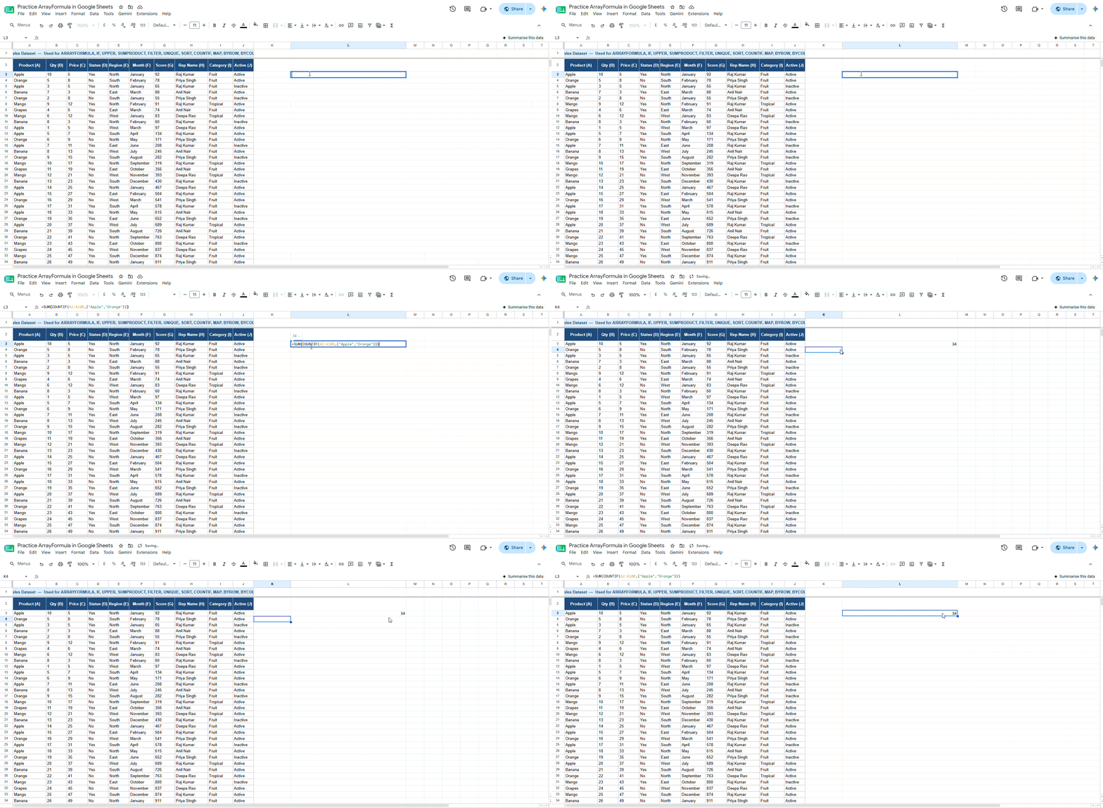
The COUNTIF function returns separate counts for each item in the array, and SUM combines those counts into one total.
This approach is especially useful when analyzing datasets that contain multiple categories, such as counting sales for several products at once without needing separate formulas for each item.
FILTER
The FILTER function in Google Sheets is used to return only the rows that match specific conditions from a dataset. For example, the formula
=FILTER(A2:D100,C2:C100="Completed") scans the range A2:D100 and displays only the rows where the corresponding value in column C is "Completed".
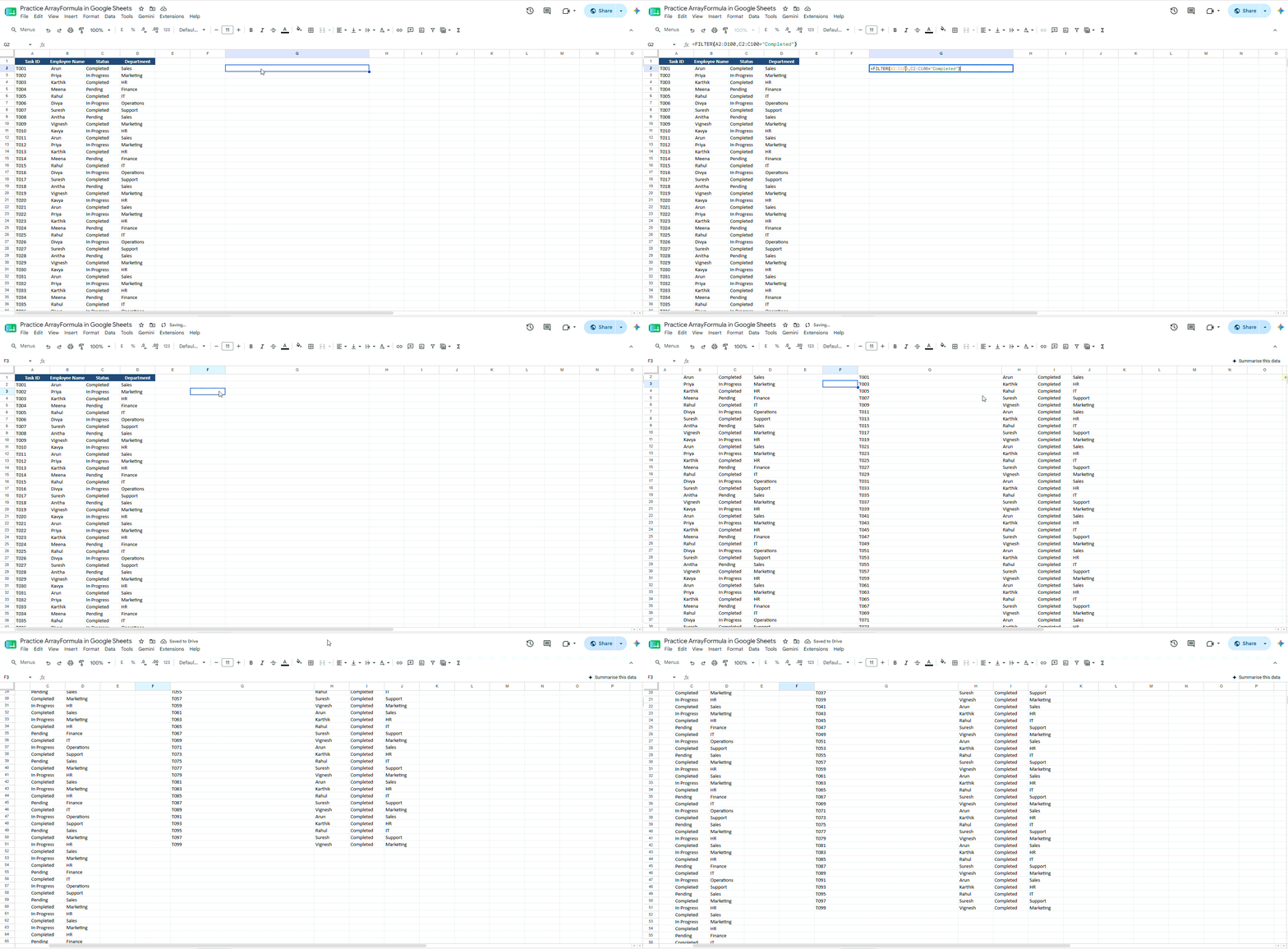
Unlike manual filtering, the results update automatically whenever the data changes, making it a powerful tool for dynamic reporting.
This function is especially useful for creating live task lists, project trackers, filtered dashboards, or automatically displaying records that meet certain criteria without modifying the original dataset.
UNIQUE
The UNIQUE function in Google Sheets is used to automatically remove duplicate values from a range and return only distinct entries.
For example, the formula =UNIQUE(A2:A100) scans the selected range and displays each value only once, regardless of how many times it appears in the original data.
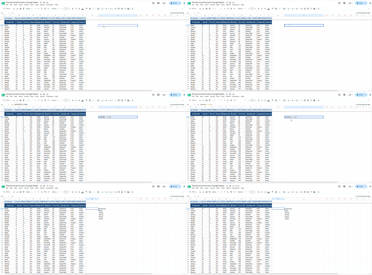
The results update dynamically whenever new data is added or existing values change. This function is especially useful for creating unique customer lists, generating category summaries, extracting distinct product names, or preparing clean datasets for analysis and reporting.
SORT
The SORT function in Google Sheets is used to organize data dynamically based on selected columns and sorting rules.
For example, the formula =SORT(A2:C100,2,FALSE) sorts the range A2:C100 using the second column as the sorting reference and arranges the data in descending order because FALSE represents descending sorting.
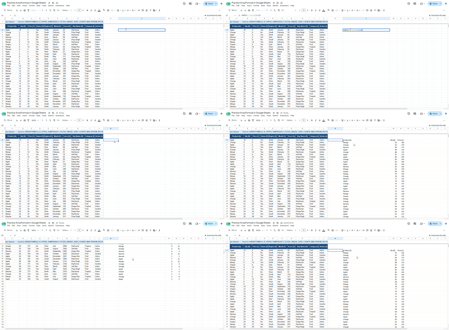
Unlike manual sorting, the results update automatically whenever the underlying data changes. This function is especially useful for ranking sales representatives by performance, organizing scores from highest to lowest, sorting inventory data, or building live dashboards that always remain up to date.
Combining FILTER, SORT, and UNIQUE
Google Sheets formulas become even more powerful when multiple array functions are combined.
For example, the formula =SORT(UNIQUE(FILTER(A2:A100,B2:B100="Active"))) first uses FILTER to return only the entries where column B contains "Active". Then, UNIQUE removes any duplicate values from the filtered results, and finally, SORT arranges the remaining values in alphabetical order automatically.
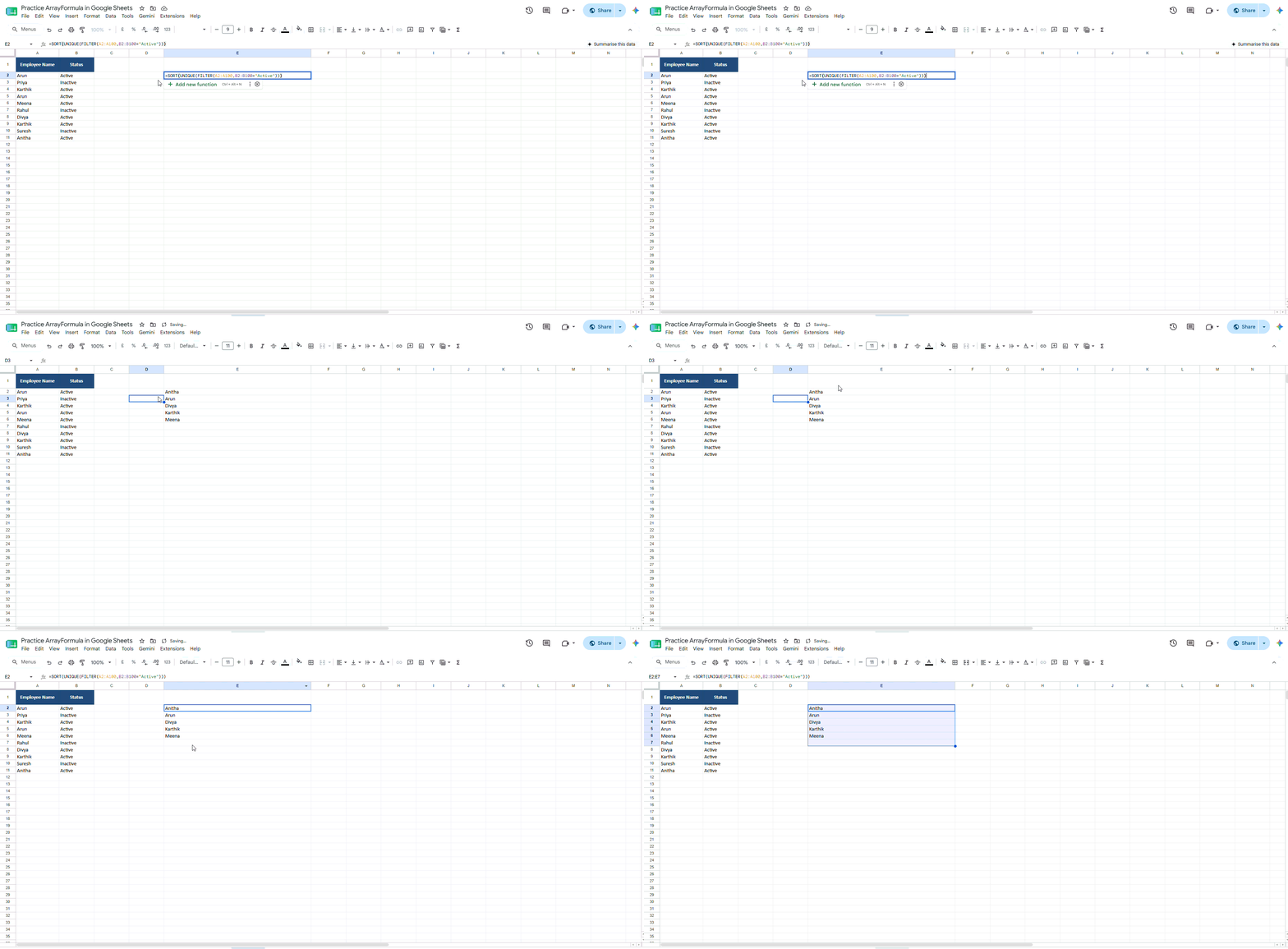
This creates a clean, dynamic list that updates instantly whenever the source data changes. Such combined formulas are especially useful for building dynamic dropdown lists, generating summary reports, organizing active customer records, or creating automated dashboards with minimal manual work.
Building Conditions into Arrays
Understanding Boolean Arrays
Boolean arrays use TRUE and FALSE values inside formulas.
In Google Sheets:
- TRUE behaves like 1
- FALSE behaves like 0
This allows conditions to be multiplied or added together mathematically.
AND Logic with *
Using * means all conditions must be true.
Formula: =FILTER(A2:D100,(B2:B100="North")*(C2:C100="January"))
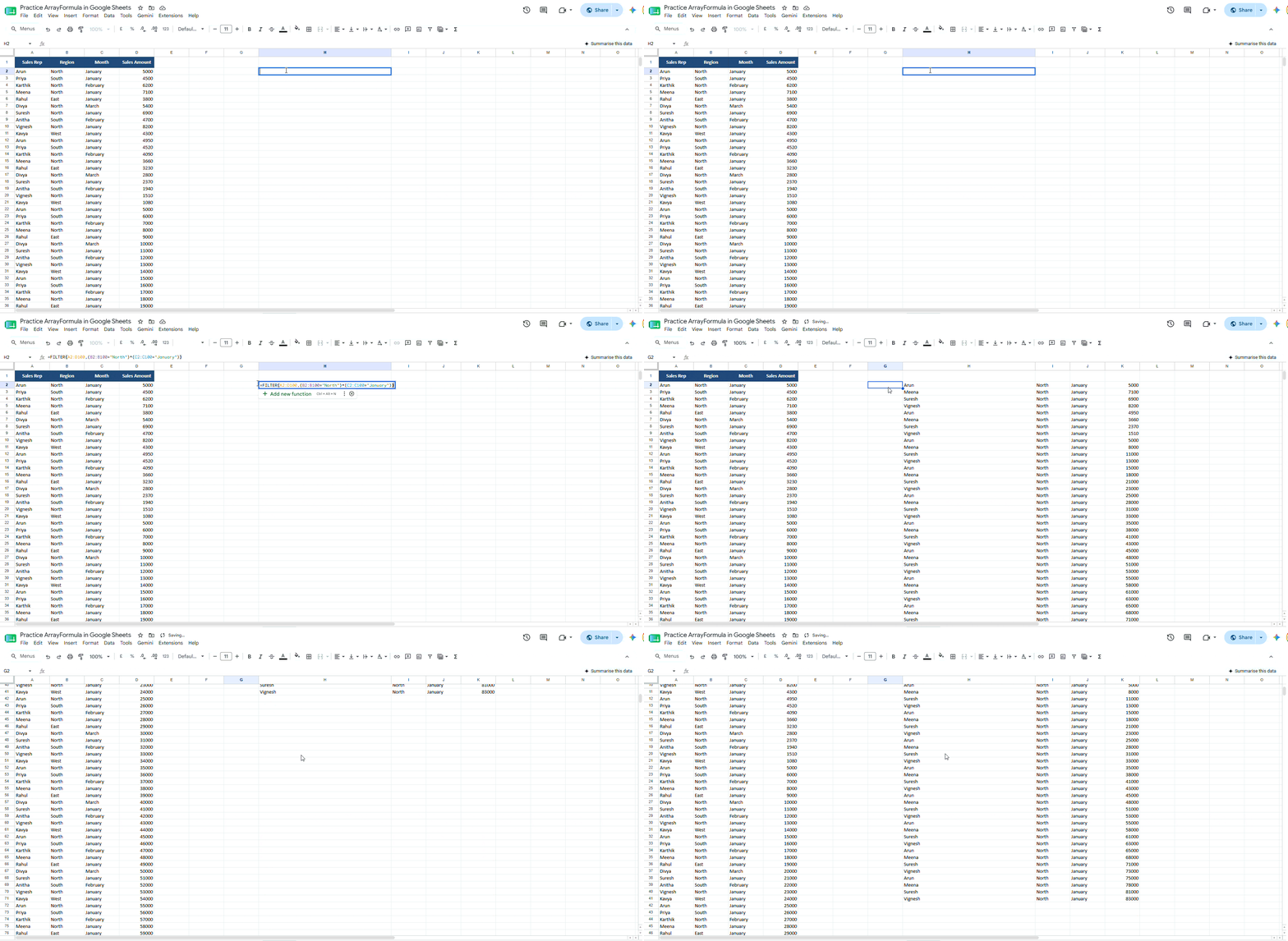
What it does: Returns rows where the region is North and the month is January.
Use case: Filtering regional sales reports by month.
OR Logic with +
Using + means at least one condition must be true.
Formula: =FILTER(A2:D100,(B2:B100="North")+(B2:B100="South"))
What it does: Returns rows from either the North or South region.
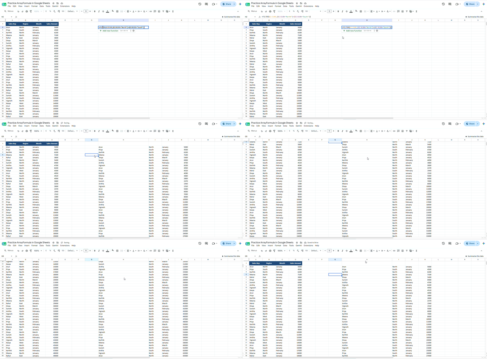
Use case: Building flexible reporting filters.
Advanced Array Techniques
MMULT for Matrix Calculations
MMULT performs matrix multiplication.
Formula: =MMULT(A2:C4,E2:G4)
What it does: Multiplies two matrices together.
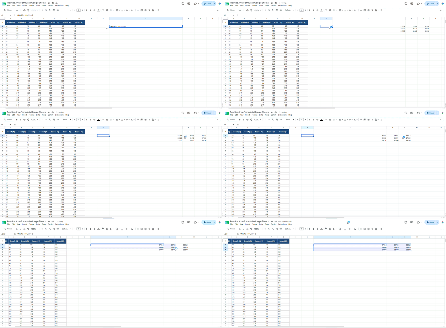
Use case: Financial modeling, engineering calculations, or weighted scoring systems.
Row-Wise Summing with MMULT
Formula: =MMULT(A2:D100,{1;1;1;1})
What it does: Sums every row across four columns automatically.
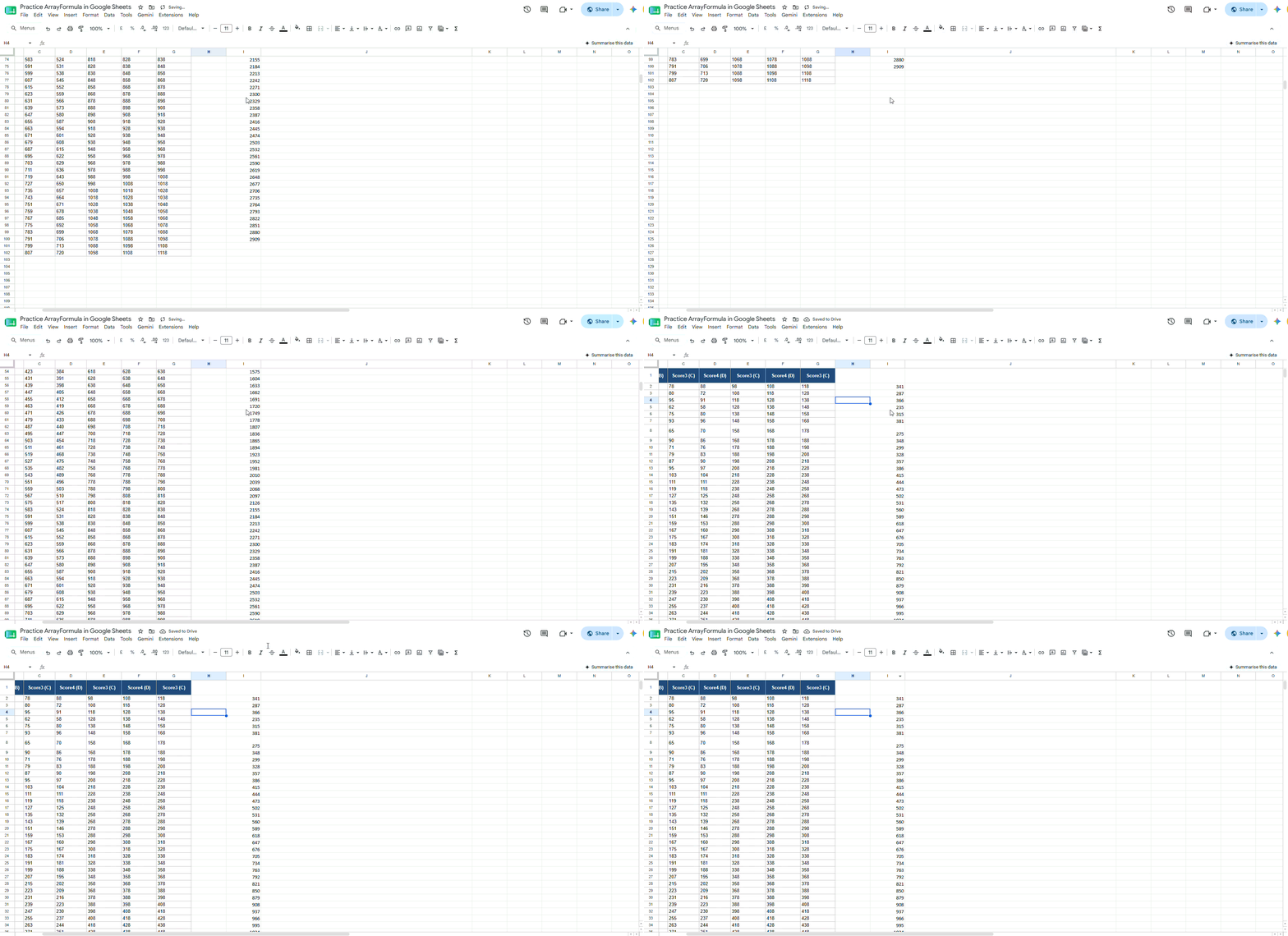
Use case: Calculating total scores across multiple evaluation categories.
MAP and LAMBDA
MAP applies custom logic to every value in an array.
Formula: =MAP(A2:A10,LAMBDA(x,x*1.1))
What it does: Multiplies every value by 1.1 individually.
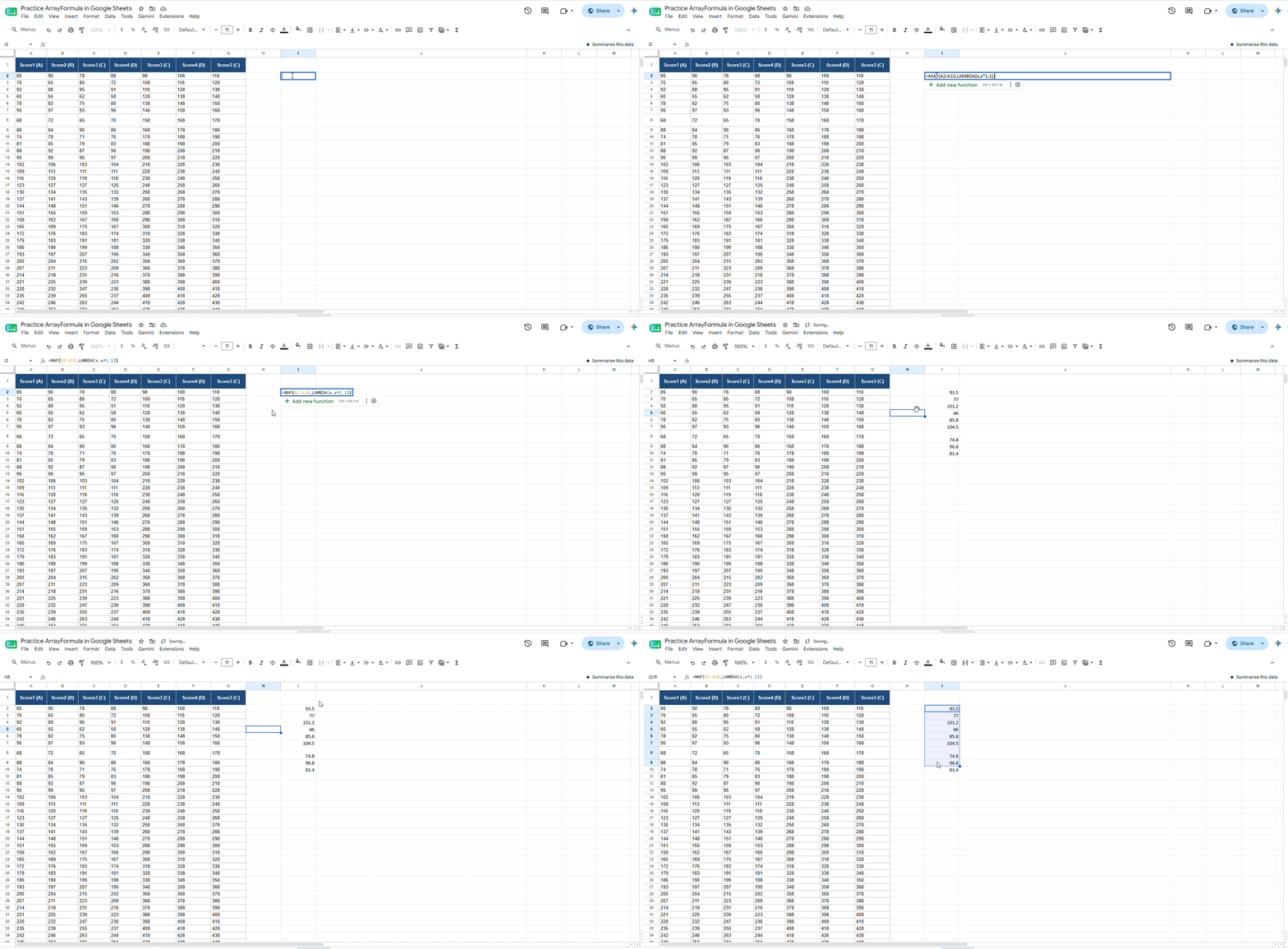
Use case: Applying tax, commission, or markup calculations dynamically.
BYROW
BYROW processes one row at a time.
Formula: =BYROW(A2:D10,LAMBDA(r,SUM(r)))
What it does: Sums each row independently.
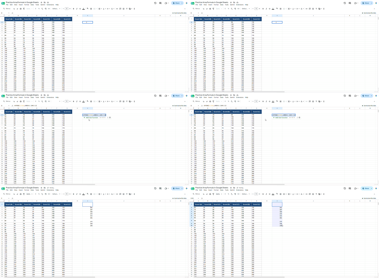
Use case: Generating row-wise totals without helper columns.
BYCOL
BYCOL processes columns individually.
Formula: =BYCOL(A1:D100,LAMBDA(c,AVERAGE(c)))
What it does: Calculates the average of each column.
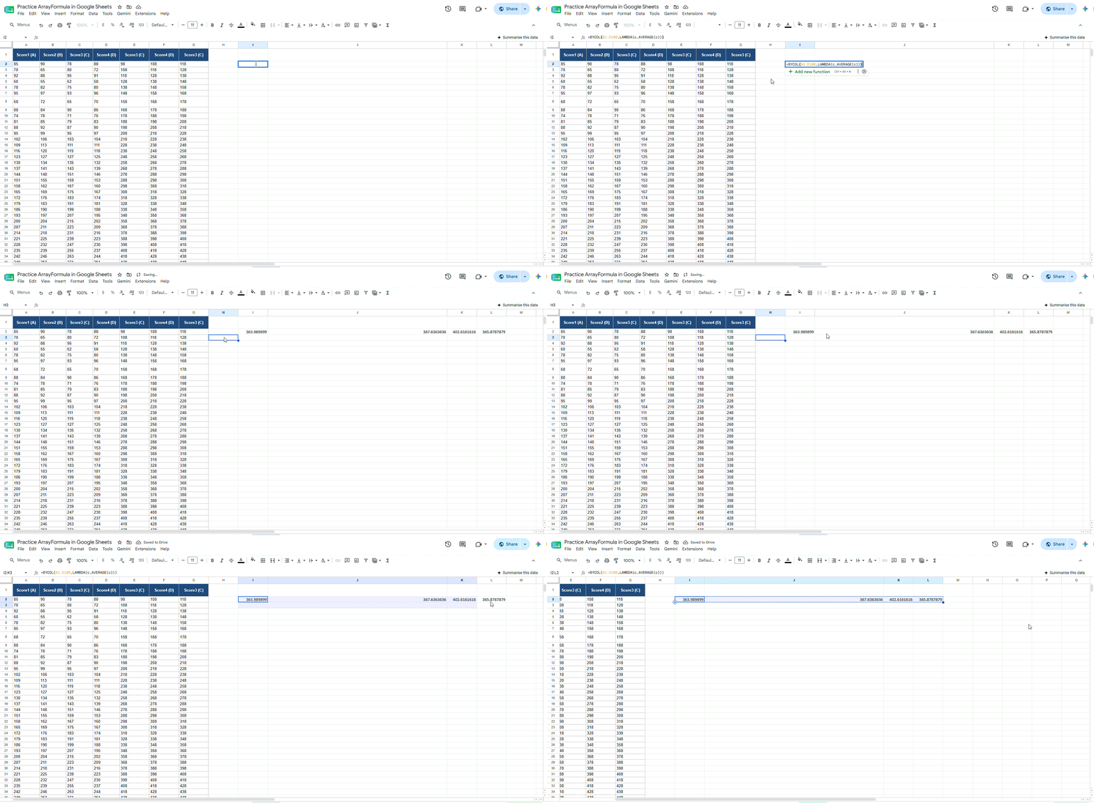
Use case: Building summary statistics tables automatically.
Nested IF with Arrays
Formula: =ARRAYFORMULA(IF(B2:B100>=90,"A",IF(B2:B100>=75,"B","C")))
What it does: Assigns grades automatically based on score ranges.
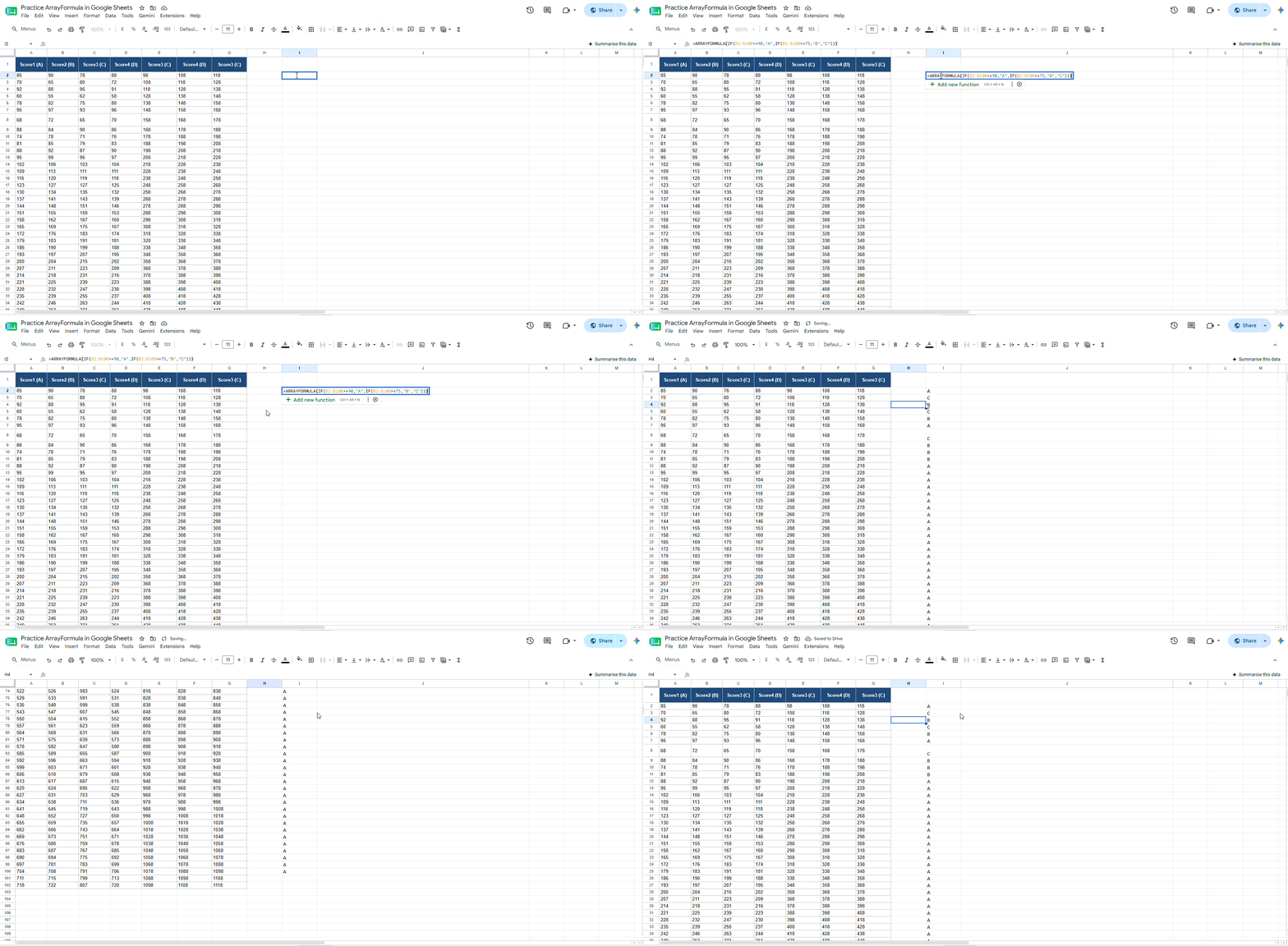
Use case: Student grading systems or employee evaluations.
Using IFS Inside Arrays
Formula:
=ARRAYFORMULA(IFS(B2:B100>=90,"Excellent",B2:B100>=75,"Good",B2:B100<75,"Needs Improvement"))
What it does: Evaluates multiple conditions across an entire range.
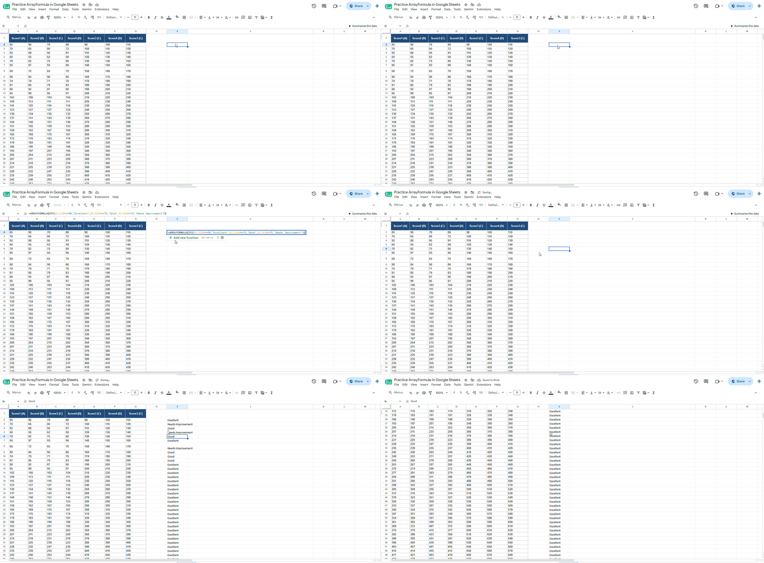
Use case: Performance review categorization.
Pro Tips for Working with Array Formulas
- Always leave empty rows and columns below array outputs so the formula can expand properly without spill errors.
- Use IFERROR to suppress unnecessary blank or error outputs.
- Example: =IFERROR(ARRAYFORMULA(A2:A100/B2:B100),"")
- Avoid volatile functions like TODAY(), NOW(), and RAND() inside large array formulas because they recalculate constantly and can slow down your spreadsheet.
- Use open-ended ranges carefully. A range like A2:A is convenient, but using it across thousands of rows can affect performance in complex spreadsheets.
- Break very large formulas into helper columns when troubleshooting. It makes debugging much easier.
Common Mistakes to Avoid [Beginner to Advanced]
- Forgetting to wrap multi-row calculations inside ARRAYFORMULA, causing only the first row to calculate.
- Hardcoding ranges like A2:A100 when your dataset regularly grows beyond row 100.
- Confusing curly brace literal arrays {} with automatic dynamic array outputs.
- Placing manual data inside the output range of an array formula, which causes expansion errors.
- Using complicated array formulas when a Pivot Table or simple filter would solve the problem more cleanly.
Conclusion
Array formulas completely change how you work in Google Sheets. What starts as a simple way to avoid dragging formulas down can eventually grow into advanced spreadsheet automation. You can calculate entire columns instantly, build dynamic filters, create intelligent summaries, and even design spreadsheet systems that update themselves automatically.
The best way to learn array formulas is through practice. Start small with ARRAYFORMULA, then experiment with FILTER, SUMPRODUCT, BYROW, and MAP. Over time, you will begin thinking in ranges and datasets instead of individual cells.
Once your Google Sheets formulas start generating useful insights, you'll want an easier way to share and understand them. ChartApps helps by converting spreadsheet data into interactive charts and dashboards, making reporting simpler and more engaging for everyone involved.